50. dynamics

50.1 Introduction to dynamics

The additional package dynamics includes several functions to create various graphical representations of discrete dynamical systems and fractals, and an implementation of the Runge-Kutta 4th-order numerical method for solving systems of differential equations.

To use the functions in this package you must first load it with load("dynamics").

Changes introduced in Maxima 5.12

Starting with Maxima 5.12, the dynamics package now uses the function plot2d to do the graphs. The commands that produce graphics (with the exception of julia and mandelbrot) now accept any options of plot2d, including the option to change among the various graphical interfaces, using different plot styles and colors, and representing one or both axes in a logarithmic scale. The old options domain, pointsize, xcenter, xradius, ycenter, yradius, xaxislabel and yaxislabel are not accepted in this new version.

All programs will now accept any variables names, and not just x and y as in the older versions. Two required parameters have changes in two of the programs: evolution2d now requires a list naming explicitely the two independent variables, and the horizontal range for orbits no longer requires a step size; the range should only specify the variable name, and the minimum and maximum values; the number of steps can now be changed with the option nticks.

50.2 Functions and Variables for dynamics

Function: chaosgame ([[x1, y1]...[xm, ym]], [x0, y0], b, n, ..., options, ...);

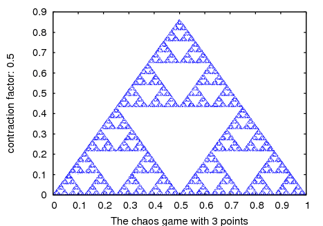
Implements the so-called chaos game: the initial point (x0, y0) is plotted and then one of the m points [x1, y1]...[xm, ym] will be selected at random. The next point plotted will be on the segment from the previous point plotted to the point chosen randomly, at a distance from the random point which will be b times that segment's length. The procedure is repeated n times.

Categories:  Package dynamics Plotting

Function: evolution (F, y0, n, ..., options, ...);

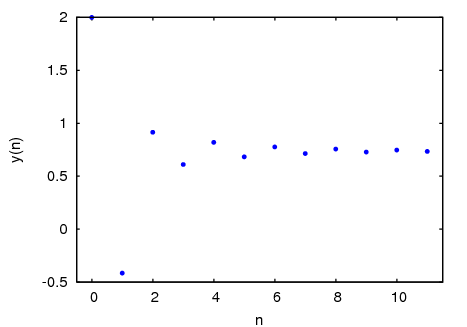
Draws n+1 points in a two-dimensional graph, where the horizontal coordinates of the points are the integers 0, 1, 2, ..., n, and the vertical coordinates are the corresponding values y(n) of the sequence defined by the recurrence relation

        y(n+1) = F(y(n))

With initial value y(0) equal to y0. F must be an expression that depends only on one variable (in the example, it depend on y, but any other variable can be used), y0 must be a real number and n must be a positive integer.

Categories:  Package dynamics Plotting

Function: evolution2d ([F, G], [u, v], [u0, y0], n, ..., options, ...);

Shows, in a two-dimensional plot, the first n+1 points in the sequence of points defined by the two-dimensional discrete dynamical system with recurrence relations

        u(n+1) = F(u(n), v(n))    v(n+1) = G(u(n), v(n))

With initial values u0 and v0. F and G must be two expressions that depend only on two variables, u and v, which must be named explicitely in a list.

Categories:  Package dynamics Plotting

Function: ifs ([r1, ..., rm], [A1, ..., Am], [[x1, y1], ..., [xm, ym]], [x0, y0], n, ..., options, ...);

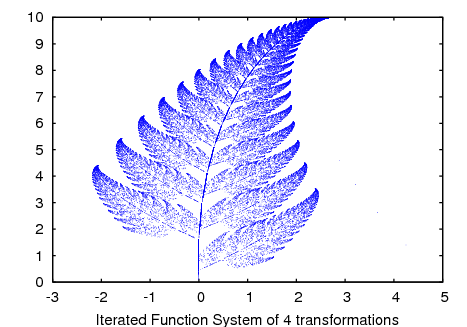
Implements the Iterated Function System method. This method is similar to the method described in the function chaosgame, but instead of shrinking the segment from the current point to the randomly chosen point, the 2 components of that segment will be multiplied by the 2 by 2 matrix Ai that corresponds to the point chosen randomly.

The random choice of one of the m attractive points can be made with a non-uniform probability distribution defined by the weights r1,...,rm. Those weights are given in cumulative form; for instance if there are 3 points with probabilities 0.2, 0.5 and 0.3, the weights r1, r2 and r3 could be 2, 7 and 10.

Categories:  Package dynamics Plotting

Function: julia (x, y, ...options...)

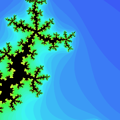
Creates a graphics file with the representation of the Julia set for the complex number (x + i y). The parameters x and y must be real. The file is created in the current directory or in the user's directory, using the XPM graphics format. The program may take several seconds to run and after it is finished, a message will be printed with the name of the file created.

The points which do not belong to the Julia set are assigned different colors, according to the number of iterations it takes the sequence starting at that point to move out of the convergence circle of radius 2. The maximum number of iterations is set with the option levels; after that number of iterations, if the sequence is still inside the convergence circle, the point will be painted with the color defined by the option color.

All the colors used for the points that do not belong to the Julia set will have the same saturation and value, but with different hue angles distributed uniformly between hue and (hue + huerange).

options is an optional sequence of options. The list of accepted options is given in a section below.

Categories:  Package dynamics Plotting

Function: mandelbrot (options)

Creates a graphics file with the representation of the Mandelbrot set. The file is created in the current directory or in the user's directory, using the XPM graphics format. The program may take several seconds to run and after it is finished, a message will be printed with the name of the file created.

The points which do not belong to the Mandelbrot set are assigned different colors, according to the number of iterations it takes the sequence generated with that point to move out of the convergence circle o radius 2. The maximum number of iterations is set with the option levels; after that number of iterations, if the sequence is still inside the convergence circle, the point will be painted with the color defined by the option color.

All the colors used for the points that do not belong to the Mandelbrot set will have the same saturation and value, but with different hue angles distributed uniformly between hue and (hue + huerange).

options is an optional sequence of options. The list of accepted options is given in a section below.

Categories:  Package dynamics Plotting

Function: orbits (F, y0, n1, n2, [x, x0, xf, xstep], ...options...);

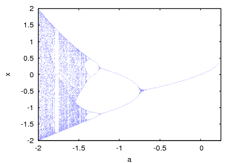
Draws the orbits diagram for a family of one-dimensional discrete dynamical systems, with one parameter x; that kind of diagram is used to study the bifurcations of a one-dimensional discrete system.

The function F(y) defines a sequence with a starting value of y0, as in the case of the function evolution, but in this case that function will also depend on a parameter x that will take values in the interval from x0 to xf with increments of xstep. Each value used for the parameter x is shown on the horizontal axis. The vertical axis will show the n2 values of the sequence y(n1+1),..., y(n1+n2+1) obtained after letting the sequence evolve n1 iterations.

Categories:  Package dynamics Plotting

Function: staircase (F, y0, n, ...options...);

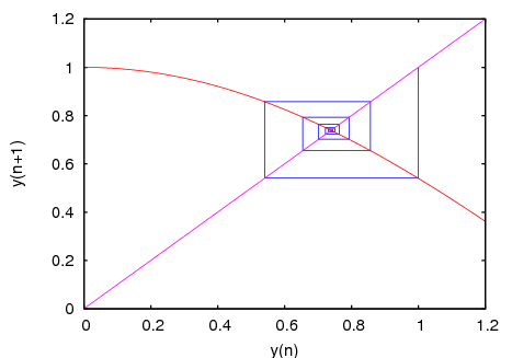
Draws a staircase diagram for the sequence defined by the recurrence relation

        y(n+1) = F(y(n))

The interpretation and allowed values of the input parameters is the same as for the function evolution. A staircase diagram consists of a plot of the function F(y), together with the line G(y) = y. A vertical segment is drawn from the point (y0, y0) on that line until the point where it intersects the function F. From that point a horizontal segment is drawn until it reaches the point (y1, y1) on the line, and the procedure is repeated n times until the point (yn, yn) is reached.

Categories:  Package dynamics Plotting

Options

Each option is a list of two or more items. The first item is the name of the option, and the remainder comprises the arguments for the option.

The options accepted by the functions evolution, evolution2d, staircase, orbits, ifs and chaosgame are the same as the options for plot2d. In addition to those options, orbits accepts and extra option pixels that sets up the maximum number of different points that will be represented in the vertical direction.

The following options are accepted by the functions julia and mandelbrot:

• size takes either one or two arguments. If only one argument is given, the width and height of the graphic file created will be equal to that value, in pixels. If two arguments are given, they will define the width and height. The default value is 400 pixels for both the width and height. If the two values are not equal, the set will appear distorted.
• levels defines the maximum number of iterations, which is also equal to the number of colors used for points not belonging to the set. The default value is 12; larger values mean much longer processing times.
• huerange defines the range of hue angles used for the hue of points not belonging to the set. The default value is 360, which means that the colors will expand all the range of hues. Values bigger than 360, will mean repeated ranges of the hue, and negative values can be used to make the hue angle decrease as the number of iterations increases.
• hue sets the hue, in degrees, of the first color used for the points which do not belong to the set. Its default value is 300 degrees, which corresponds to magenta; the values for other standard colors are 0 for red, 45 for orange, 60 for yellow, 120 for green, 180 for cyan and 240 for blue. See also option huerange.
• saturation sets the value of the saturation used for points not belonging to the set. It must be between 0 and 1. The default is 0.46.
• value sets the value of the colors used for points not belonging to the set. It must be between 0 and 1; the higher the value, the brighter the colors. The default is 0.96
• color must be followed by three parameters that define the hue, saturation and value, for the color used to represent the points of the set. The default value is 0 for the three parameters, which corresponds to black. For an explanation of the range of allowed values, see options hue, saturation and value.
• center must be followed by two real parameters, which give the coordinates, on the complex plane, of the point in the center of the region shown. The default value is 0 for both coordinates (the origin).
• radius sets the radius of the biggest circle inside the square region that will be displayed. The default value is 2.
• filename gives the name of the file where the resulting graph will be saved. The extension .xpm will be added to that name. If the file already exists, it will be replaced by the file generated by the function. The default values are julia for the Julia set, and mandelbrot for the Mandelbrot set.

Examples

Graphical representation and staircase diagram for the sequence: 2, cos(2), cos(cos(2)),...

(%i1) load("dynamics")$

(%i2) evolution(cos(y), 2, 11);

(%i3) staircase(cos(y), 1, 11, [y, 0, 1.2]);

If your system is slow, you'll have to reduce the number of iterations in the following examples. And if the dots appear too small in your monitor, you might want to try a different style, such as [style,[points,0.8]].

Orbits diagram for the quadratic map, with a parameter a.

        x(n+1) = a + x(n)^2

(%i4) orbits(x^2+a, 0, 50, 200, [a, -2, 0.25], [style, dots]);

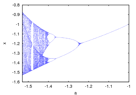
To enlarge the region around the lower bifurcation near x = -1.25 use:

(%i5) orbits(x^2+a, 0, 100, 400, [a,-1,-1.53], [x,-1.6,-0.8],
             [nticks, 400], [style,dots]);

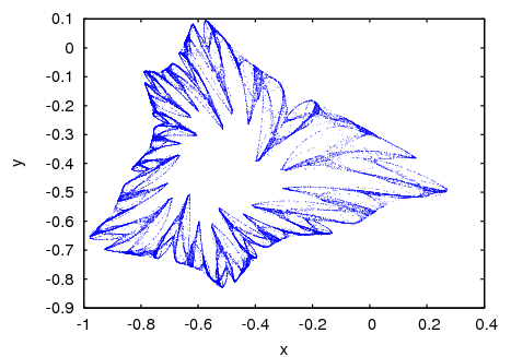
Evolution of a two-dimensional system that leads to a fractal:

(%i6) f: 0.6*x*(1+2*x)+0.8*y*(x-1)-y^2-0.9$

(%i7) g: 0.1*x*(1-6*x+4*y)+0.1*y*(1+9*y)-0.4$

(%i8) evolution2d([f,g], [x,y], [-0.5,0], 50000, [style,dots]);

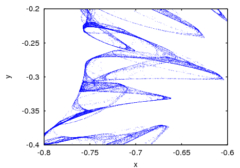
And an enlargement of a small region in that fractal:

(%i9) evolution2d([f,g], [x,y], [-0.5,0], 300000, [x,-0.8,-0.6],
                  [y,-0.4,-0.2], [style, dots]);

A plot of Sierpinsky's triangle, obtained with the chaos game:

(%i9) chaosgame([[0, 0], [1, 0], [0.5, sqrt(3)/2]], [0.1, 0.1], 1/2,
                 30000, [style, dots]);

Barnsley's fern, obtained with an Iterated Function System:

(%i10) a1: matrix([0.85,0.04],[-0.04,0.85])$

(%i11) a2: matrix([0.2,-0.26],[0.23,0.22])$

(%i12) a3: matrix([-0.15,0.28],[0.26,0.24])$

(%i13) a4: matrix([0,0],[0,0.16])$

(%i14) p1: [0,1.6]$

(%i15) p2: [0,1.6]$

(%i16) p3: [0,0.44]$

(%i17) p4: [0,0]$

(%i18) w: [85,92,99,100]$

(%i19) ifs(w, [a1,a2,a3,a4], [p1,p2,p3,p4], [5,0], 50000, [style,dots]);

To create a file named dynamics9.xpm with a graphical representation of the Mandelbrot set, with 12 colors, use:

mandelbrot([filename,"dynamics9"])$

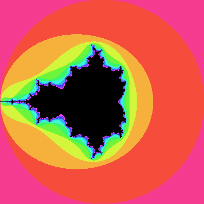
and the Julia set for the number (-0.55 + i 0.6) can be obtained with:

julia(-0.55, 0.6, [levels, 36], [center, 0, 0.6], [radius, 0.3],
      [hue, 240], [huerange, -180], [filename, "dynamics10"])$

the graph will be saved in the file dynamics10.xpm and will show the region from -0.3 to 0.3 in the x direction, and from 0.3 to 0.9 in the y direction. 36 colors will be used, starting with blue and ending with yellow.

This document was generated by Charlie & on July, 6 2015 using texi2html 1.76.