Extended LaTeXModule for Sympy
| Author: | Alan Bromborsky |
|---|
Abstract
This document describes the extension of the latex module for sympy. The python module latex_ex extends the capabilities of the current latex (while preserving the current capabilities) to geometric algebra multivectors, numpy array’s, and extends the ascii formatting of greek symbols, accents, and subscripts and superscripts. Additionally the module is configured to use the print command to generate a LaTeX output file and display it using xdvi in Linux and yap in Windows. To get LaTeX displayed text latex and xdvi must be installed on a Linux system and MikTex on a Windows system.
Extended Symbol Coding
One of the main extensions in latex_ex is the ability to encode complex symbols (multiple greek letters with accents and superscripts and subscripts) is ascii strings containing only letters, numbers, and underscores. These restrictions allow sympy variable names to represent complex symbols. For example if we use the GA module function make_symbols() as follows:
make_symbols('xalpha Gammavec__1_rho delta__j_k')
make_symbols creates the three sympy symbols xalpha, Gammavec__1_rho, and delta__j_k. If these symbols are printed with the latex_ex modules the results are
Ascii String |
LaTeX Output |
|---|---|
xalpha |
|
Gammavec__1_rho |
|
delta__j_k |


A single underscore denotes a subscript and a double undscore a superscript.
In addition to all normal LaTeX accents boldmath is supported so that
omegaomegabm so an accent (or boldmath)
only applies to the character (characters in the case of the string representing
a greek letter) immediately preceeding the accent command.
so an accent (or boldmath)
only applies to the character (characters in the case of the string representing
a greek letter) immediately preceeding the accent command.
How LatexPrinter Works
The actual LatexPrinter class is hidden with the helper functions Format(), LaTeX(), and xdvi(). LatexPrinter is setup when Format() is called. In addition to setting format switches in LatexPrinter, Format() does two other critical tasks. Firstly, the sympy function Basic.__str__() is redirected to the LatexPrinter helper function LaTeX(). If nothing more that this were done the python print command would output LaTeX code. Secondly, sys.stdout is redirected to a file until xdvi() is called. This file is then compiled with the latex program (if present) and the dvi output file is displayed with the xdvi program (if present). Thus for LatexPrinter to display the output in a window both latex and xdvi must be installed on your system and in the execution path.
One problem for LatexPrinter is determining when equation mode should be use in the output formatting. To allow for printing output not in equation mode the program attemps to determine from the output string context when to use equation mode. The current test is to use equation mode if the string contains an =, _, ^, or \. This is not a foolproof method. The safest thing to do if you wish to print an object, X, in math mode is to use print ‘X =’,X so the = sign triggers math mode.
LatexPrinter Functions
LatexPrinter Class Functions for Extending LatexPrinter Class
The LatexPrinter class functions are not called directly, but rather are called when print(), LaTeX(), or str() are called. The two new functions for extending the latex module are _print_ndarray() and _print_MV(). Some other functions in LatexPrinter have been modified to increase their utility.
- _print_ndarray(self, expr)
- _print_ndarray() returns a latex formatted string for the expr equal to a numpy array with elements that can be sympy expressions. The numpy array’s can have up to three dimensions.
- _print_MV(self, expr)
- _print_MV() returns a latex formatted string for the expr equal to a GA multivector.
- str_basic(in_str)
- str_basic() returns a string without the latex formatting provided by LatexPrinter. This is needed since LatexPrinter takes over the str() fuction and there are instances when the unformatted string is needed such as during the automatic generation of multivector coefficients and the reduction of multivector coefficients for printing.
Helper Functions for Extending LatexPrinter Class
- Format(fmt='1 1 1 1')
Format iniailizes LatexPrinter and set the format for sympy symbols, functions, and derivatives and for GA multivectors. The switch are encoded in the text string argument of Format as follows. It is assumed that the text string fmt always contains four integers separated by blanks.
Position
Switch
Values

symbol
0: Use symbol encoding in latex.py
1: Use extended symbol encoding in latex_ex.py

function
0: Use symbol encoding in latex.py. Print functions args, use \operator{ } format.
1: Do not print function args. Do not use \operator{} format. Suppress printing of function arguments.

partial derivative
0: Use partial derivative format in latex.py.
1: Use format
 instead of
  .
.
multivector
1: Print entire multivector on one line.
2: Print each grade of multivector on one line.
3: Print each base of multivector on one line.
- LaTeX(expr, inline=True)
LaTeX() returns the latex formatted string for the sympy, GA, or numpy expression expr. This is needed since numpy cannot be subclassed and hence cannot be used with the LatexPrinter modified print() command. Thus is A is a numpy array containing sympy expressions one cannot simply code
print A
but rather must use
print LaTeX(A)
- xdvi(filename='tmplatex.tex', debug=False)
- xdvi() postprocesses the output of the print statements and generates the latex file with name filename. If the latex and xdvi programs are present on the system they are invoked to display the latex file in a window. If debug=True the associated output of latex is sent to stdout, otherwise it is sent to /dev/null for linux and NUL for Windows. If LatexPrinter has not been initialized xdvi() does nothing. After the .dvi file is generated it is displayed with xdvi for linux (if latex and xdvi are installed ) and yap for Windows (if MikTex is installed).
The functions sym_format(), fct_format(), pdiff_format(), and MV_format() allow one to change various formatting aspects of the LatexPrinter. They do not initialize the class and if the are called with the class not initialized they have no effect. These functions and the function xdvi() are designed so that if the LatexPrinter class is not initialized the program output is as if the LatexPrinter class is not used. Thus all one needs to do to get simple ascii output (possibly for program debugging) is to comment out the one function call that initializes the LatexPrinter class. All other latex_ex function calls can remain in the program and have no effect on program output.
- sym_format(sym_fmt)
- sym_format() allows one to change the latex format options for
sympy symbol output independent of other format switches (see
switch in Table I).
- fct_format(fct_fmt)
- fct_format() allows one to change the latex format options for
sympy function output independent of other format switches (see
switch in Table I).
- pdiff_format(pdiff_fmt)
- pdiff_format() allows one to change the latex format options for
sympy partial derivative output independent of other format switches
(see switch in Table I).
- MV_format(mv_fmt)
- MV_format() allows one to change the latex format options for
sympy partial derivative output independent of other format switches
(see switch in Table I).
Examples
latexdemo.py a simple example
latexdemo.py example of using latex_ex with sympy
import sys
import sympy.galgebra.GA as GA
import sympy.galgebra.latex_ex as tex

GA.set_main(sys.modules[__name__])

if __name__ == '__main__':

    tex.Format()
    GA.make_symbols('xbm alpha_1 delta__nugamma_r')

    x = alpha_1*xbm/delta__nugamma_r

    print 'x =',x

    tex.xdvi()
Start of Program Output

End of Program Output
The program latexdemo.py demonstrates the extended symbol naming
conventions in latex_ex. the statment Format() starts the
LatexPrinter driver with default formatting. Note that on the right
hand side of the output that xbm gives  , alpha_1 gives
 and delta__nugamma_r gives
  .
Also the fraction is printed correctly. The statment print 'x =',x sends
the string 'x = '+str(x) to the output processor (xdvi()). Because
the string contains an
.
Also the fraction is printed correctly. The statment print 'x =',x sends
the string 'x = '+str(x) to the output processor (xdvi()). Because
the string contains an  sign the processor treats the string as an
LaTeX equation (unnumbered). If 'x =' was not in the print statment a
LaTeX error would be generated. In the case of a GA multivector one
does not need the 'x =' if the multivector has been given a name. In the
example the GA function make_symbols() has been used to create
the sympy symbols for convenience. The sympy function
Symbol() could have also been used.
sign the processor treats the string as an
LaTeX equation (unnumbered). If 'x =' was not in the print statment a
LaTeX error would be generated. In the case of a GA multivector one
does not need the 'x =' if the multivector has been given a name. In the
example the GA function make_symbols() has been used to create
the sympy symbols for convenience. The sympy function
Symbol() could have also been used.
Maxwell.py a multivector example
Maxwell.py example of using latex_ex with GA
import sys
import sympy.galgebra.GAsympy as GA
import sympy.galgebra.latex_ex as tex
GA.set_main(sys.modules[__name__])
if __name__ == '__main__':
metric = '1 0 0 0,'+\
'0 -1 0 0,'+\
'0 0 -1 0,'+\
'0 0 0 -1'
vars = GA.make_symbols('t x y z')
GA.MV.setup('gamma_t gamma_x gamma_y gamma_z',metric,True,vars)
tex.Format()
I = GA.MV(1,'pseudo')
I.convert_to_blades()
print '$I$ Pseudo-Scalar'
print 'I =',I
B = GA.MV('B','vector',fct=True)
E = GA.MV('E','vector',fct=True)
B.set_coef(1,0,0)
E.set_coef(1,0,0)
B *= gamma_t
E *= gamma_t
B.convert_to_blades()
E.convert_to_blades()
J = GA.MV('J','vector',fct=True)
print '$B$ Magnetic Field Bi-Vector'
print 'B = Bvec gamma_0 =',B
print '$E$ Electric Field Bi-Vector'
print 'E = Evec gamma_0 =',E
F = E+I*B
print '$E+IB$ Electo-Magnetic Field Bi-Vector'
print 'F = E+IB =',F
print '$J$ Four Current'
print 'J =',J
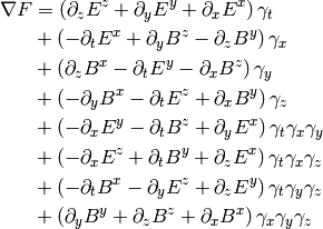
gradF = F.grad()
gradF.convert_to_blades()
print 'Geometric Derivative of Electo-Magnetic Field Bi-Vector'
tex.MV_format(3)
print '\\nabla F =',gradF
print 'All Maxwell Equations are'
print '\\nabla F = J'
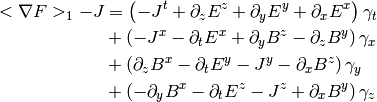
print 'Div $E$ and Curl $H$ Equations'
print '<\\nabla F>_1 -J =',gradF.project(1)-J,' = 0'
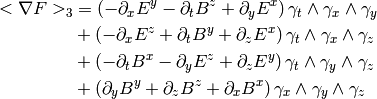
print 'Curl $E$ and Div $B$ equations'
print '<\\nabla F>_3 =',gradF.project(3),' = 0'
tex.xdvi(filename='Maxwell.tex')
Start of Program Output
 Pseudo-Scalar

 Magnetic Field Bi-Vector

 Electric Field Bi-Vector

 Electo-Magnetic Field Bi-Vector

 Four Current

Geometric Derivative of Electo-Magnetic Field Bi-Vector
All Maxwell Equations are

Div  and Curl
  Equations

Curl and Div equations
End of Program Output
The program Maxwell.py demonstrates the use of the
LatexPrinter class with the GA module multivector class,
MV. The Format() call initializes LatexPrinter. The
only other explicit latex_x module formatting statement used is
MV_format(3). This statment changes the multivector latex format so that
instead of printing the entire multivector on one line, which would run off the
page, each multivector base and its coefficient are printed on individual lines
using the latex align environment. Another option used is that the printing of
function arguments is suppressed since , , , and
are multivector fields and printing out the argument,
 , for every field component would greatly lengthen the output
and make it more difficult to format in a pleasing way.
, for every field component would greatly lengthen the output
and make it more difficult to format in a pleasing way.

Table Of Contents
Previous topic
Geometric Algebra Module for Sympy